
사용한 모델의 코드와 파라미터는 아래 github을 참고해주세요.
drug_toxicity_prediction/Deep learning Classification code Pattern (Drug Toxicity Prediction)/Deep learning Classification code
Contribute to Yg-Hong/drug_toxicity_prediction development by creating an account on GitHub.
github.com
ADME
Absorption(흡수), Distribution(분포), Metabolism(대사), Excretion(배설)의 앞글자를 따와 만든 ADME는 하나의 약물이 생체 내 목표하는 장기에 이르기까지의 처리되는 과정이다. 이제 Classification 과정을 통해 ADME에서 독성률을 판단하고 위양성, 위음성률을 확인하며 모델의 성능을 검증해보자.
데이터 수집
데이터는 TCD(Therapeutics Data Commons)에서 api형태로 제공하는 Acute Toxicity LD50을 사용했다.
데이터 형태는 아래와 같다.

train data, validate data, test data는 각각 [5170 rows, 738 rows, 1477 rows] 로 약 7:1:2 비율로 split 해주었다.
데이터 전처리
화합물의 이름이나 화학 공식을 그대로 활용하기는 어렵다. 따라서 SMILES 방식으로 표현되어 있는 화합물 데이터에 대해서 RDkit의 룰베이스 방식을 활용하여 morgan fingerprint로 벡터화해줄 것이다.
from rdkit import Chem, DataStructs
from rdkit.Chem import AllChem
import numpy as np

def smiles2morgan(s, radius = 2, nBits = 1024):
    """SMILES data를 morgan fingerprint 데이터로 변환
       SMILES data가 뭐냐면? Simplified Molecular Input Line Entry System
       ex. CCCC1COC(Cn2cncn2)(c2ccc(Cl)cc2Cl)O1

    Args:
        s (str): SMILES of a drug
        radius (int): ECFP radius
        bBits (int): size of binary representation

    Return ():
        morgan fingerprint

    """
    try:
        mol = Chem.MolFromSmiles(s)
        features_vec = AllChem.GetMorganFingerprintAsBitVect(mol, radius, nBits=nBits)
        features = np.zeros((1,))
        DataStructs.ConvertToNumpyArray(features_vec, features)
    except:
        print('rdkit not found this smiles for morgan: ' + s + ' convert to all 0 features')
        features = np.zeros((nBits, ))

    return features
결과 해석
모델은 classic한 형태의 machine learning을 위한 Classification 모델을 사용했다. 사용한 모델과 파라미터는 위의 깃헙 소스코드를 참고 해달라.
# 테스트 진행

model = model_best

y_pred = []
y_label = []
y_score = []

model.eval()
for i, (v_d, label) in enumerate(valid_loader):
    # input data gpu에 올리기
    v_d = v_d.float().to(device)

    with torch.set_grad_enabled(False):
        # forward-pass
        output = model(v_d)

        # 미리 정의한 손실함수(MSE)로 손실(loss) 계산
        loss = loss_fn(output, label.to(device))

        # 각 iteration 마다 loss 기록
        loss_history_val.append(loss.item())

        pred = output.argmax(dim=1, keepdim=True)
        score = nn.Softmax(dim = 1)(output)[:,1]

        # 예측값, 참값 cpu로 옮기고 numpy 형으로 변환
        pred = pred.cpu().numpy()
        score = score.cpu().numpy()
        label = label.cpu().numpy()

    # 예측값, 참값 기록하기
    y_label = y_label + label.flatten().tolist()
    y_pred = y_pred + pred.flatten().tolist()
    y_score = y_score + score.flatten().tolist()

# metric 계산
classification_metrics = classification_report(y_label, y_pred,
                    target_names = ['NonToxic', 'Toxic'],
                    output_dict= True)
# sensitivity is the recall of the positive class
sensitivity = classification_metrics['Toxic']['recall']
# specificity is the recall of the negative class
specificity = classification_metrics['NonToxic']['recall']
# accuracy
accuracy = classification_metrics['accuracy']
# confusion matrix
conf_matrix = confusion_matrix(y_label, y_pred)
# roc score
roc_score = roc_auc_score(y_label, y_score)

# 각 epoch 마다 결과 출력
print('Validation at Epoch '+ str(epo + 1) + ' , Accuracy: ' + str(accuracy)[:7] + ' , sensitivity: '\
                        + str(sensitivity)[:7] + ' specificity: ' + str(f"{specificity}") +' , roc_score: '+str(roc_score)[:7])
훈련시킨 모델의 Test 결과는 다음과 같다.
훈련시킨 모델의 Test 결과는 다음과 같다.
Validation at Epoch 50 , Accuracy: 0.81029 , sensitivity: 0.63926 specificity: 0.882466281310212 , roc_score: 0.84503
하나하나 해석해보자.
Accuracy: 0.81029
정확도는 모델이 전체 데이터에서 예측을 얼마나 잘 맞췄는지를 나타내는 지표이다. 0.81029라는 숫자는 모델이 약 81%의 데이터를 올바르게 예측했다는 의미를 뜻한다.
Sensitivity (또는 Recall): 0.63926
민감도는 실제로 독성인 경우 중에서 모델이 독성이라고 올바르게 예측한 비율을 의미한다. 0.63926은 독성 데이터를 약 63.9% 정확도로 예측했다는 뜻이다.
Specificity: 0.882466281310212
특이도는 실제로 비독성인 경우 중에서 모델이 비독성이라고 올바르게 예측한 비율을 의미한다. 0.882466281310212은 비독성 데이터를 약 88.2% 정확도로 예측했다는 뜻이다.
ROC Score (AUC - Area Under the Curve): 0.84503
ROC 곡선의 아래 면적은 모델의 전반적인 예측 성능을 나타내는 지표이다. 0.84503이라는 값은 모델의 예측이 꽤 좋다는 것을 의미하며 1에 가까울수록 더 좋은 모델이다.
Test result visulization
테스트를 수행한 후에 결과 지표에 대해 시각화를 시도해보았다.
ROC Curve Description
- X축은 False Positive Rate (위양성률, 실제로는 비독성인데 독성이라고 예측한 비율), Y축은 True Positive Rate (민감도, 실제로 독성인 것을 독성이라고 예측한 비율)을 나타낸다.
- 곡선이 왼쪽 상단에 가까울수록 모델이 좋다는 것을 의미한다.
여기서 ROC 곡선 아래 면적(AUC)이 0.8450이므로, 모델의 예측이 꽤 좋은 편임을 뜻한다.

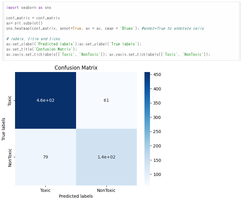
Confusion Matrix Description
- 혼동 행렬은 모델의 예측 결과를 실제 값과 비교해서 보여주는 표이다.
- "Toxic"과 "NonToxic" 두 가지 클래스를 예측했다.
- 왼쪽 위 (460): 실제로 독성인 데이터를 독성으로 맞게 예측한 경우 (True Positive).
- 오른쪽 위 (61): 실제로 독성인 데이터를 비독성으로 잘못 예측한 경우 (False Negative).
- 왼쪽 아래 (79): 실제로 비독성인 데이터를 독성으로 잘못 예측한 경우 (False Positive).
- 오른쪽 아래 (140): 실제로 비독성인 데이터를 비독성으로 맞게 예측한 경우 (True Negative).
이 혼동 행렬을 보면, 모델이 독성 데이터를 비독성으로 잘못 예측하는 경우(61)보다 비독성 데이터를 독성으로 잘못 예측하는 경우(79)가 조금 더 많다. 하지만 전반적으로 모델이 대부분의 데이터를 잘 예측하고 있다.
'의료 AI(딥러닝) 공부 일기' 카테고리의 다른 글
| CH 03-1. Covid CT image classification (0) | 2024.07.07 |
|---|---|
| CH 03-0. Deep Learning for Biomedical Image (0) | 2024.07.07 |
| CH 02-1. Drug Toxicity Prediction 응용 - Regression (0) | 2024.07.05 |
| CH 02-0. Drug Toxicity Prediction - Regression (1) | 2024.07.05 |
| Ch 01. 인공지능 헬스케어 (1) | 2024.07.05 |

댓글